Introduction to Jupyter notebooks

(c) 2021 Justin Bois. This work is licensed under a Creative Commons Attribution License CC-BY 4.0. All code contained herein is licensed under an MIT license.

This tutorial was generated from a Jupyter notebook. You can download the notebook here.

---

The first thing we'll do, discussed later, is import all the modules we'll need. You should in general do this at the very beginning of each notebook.

# Our numerical workhorses
import numpy as np
import scipy.integrate

# Plotting
import bokeh.io
import bokeh.plotting

bokeh.io.output_notebook()

Loading BokehJS ...

In this tutorial, you will learn the basics on how to use Jupyter notebooks. Your homework will be submitted as Jupyter notebooks, so this is something you will need to master. It will be useful for you to go over the introduction to LaTeX to learn how to use $\LaTeX$ in your Jupyter notebooks.

You should, of course, read the official Jupyter documentation as well.

What is Jupyter?

Jupyter is a way to combine text (with math!) and code (which runs and can display graphic output!) in an easy-to-read document that renders in a web browser. The notebook itself is stored as a text file in JSON format. This text file is what you will email the course staff when submitting your homework.

It is language agnostic as its name suggests. The name "Jupyter" is a combination of Julia (a new language for scientific computing), Python (which you know and love, or at least will when the course is over), and R (the dominant tool for statistical computation). However, you currently can run over 40 different languages in a Jupyter notebook, not just Julia, Python, and R.

Launching a Jupyter notebook

For the purposes of ChE/BE 163, you can use Jupyter either locally, or via the Amazon Machine Image we set up for you. For the latter, see the instructions in the Computing section of the course webpage. This might be the easiest way for you to use NUPACK and its Python-wrapped functions.

To launch a Jupyter notebook on your local machine, you can do the following.

• Mac: Use the Anaconda launcher and select Jupyter notebook.
• Windows: Under "Search programs and files" from the Start menu, type jupyter notebook and select "Jupyter notebook."

A Jupyter notebook will then launch in your default web browser.

You can also launch Jupyter from the command line. To do this, simply enter

jupyter notebook

on the command line and hit enter. This also allows for greater flexibility, as you can launch Jupyter with command line flags. For example, I launch Jupyter using

jupyter notebook --browser=safari

This fires up Jupyter with Safari as the browser. If you launch Jupyter from the command line, your shell will be occupied with Jupyter and will occasionally print information to the screen. After you are finished with your Jupyter session (and have saved everything), you can kill Jupyter by hitting "ctrl + C" in the terminal/PowerShell window.

When you launch Jupyter, you will be presented with a menu of files in your current working directory to choose to edit. You can also navigate around the files on your computer to find a file you wish to edit by clicking the "Upload" button in the upper right corner. You can also click "New" in the upper right corner to get a new Jupyter notebook. After selecting the file you wish to edit, it will appear in a new window in your browser, beautifully formatted and ready to edit.

Cells

A Jupyter notebook consists of cells. The two main types of cells you will use are code cells and markdown cells, and we will go into their properties in depth momentarily. First, an overview.

A code cell contains actual code that you want to run. You can specify a cell as a code cell using the pulldown menu in the toolbar in your Jupyter notebook. Otherwise, you can can hit esc and then y (denoted "esc, y") while a cell is selected to specify that it is a code cell. Note that you will have to hit enter after doing this to start editing it.

If you want to execute the code in a code cell, hit "shift + enter." Note that code cells are executed in the order you execute them. That is to say, the ordering of the cells for which you hit "shift + enter" is the order in which the code is executed. If you did not explicitly execute a cell early in the document, its results are now known to the Python interpreter.

Markdown cells contain text. The text is written in markdown, a lightweight markup language. You can read about its syntax here. Note that you can also insert HTML into markdown cells, and this will be rendered properly. As you are typing the contents of these cells, the results appear as text. Hitting "shift + enter" renders the text in the formatting you specify.

You can specify a cell as being a markdown cell in the Jupyter toolbar, or by hitting "esc, m" in the cell. Again, you have to hit enter after using the quick keys to bring the cell into edit mode.

In general, when you want to add a new cell, you can use the "Insert" pulldown menu from the Jupyter toolbar. The shortcut to insert a cell below is "esc, b" and to insert a cell above is "esc, a." Alternatively, you can execute a cell and automatically add a new one below it by hitting "alt + enter."

Code cells

Below is an example of a code cell printing hello, world. Notice that the output of the print statement appears in the same cell, though separate from the code block.

# Say hello to the world.
print('hello, world.')

hello, world.

If you evaluate a Python expression that returns a value, that value is displayed as output of the code cell. This only happens, however, for the last line of the code cell.

# Would show 9 if this were the last line, but it is not, so shows nothing
4 + 5

# I hope we see 11.
5 + 6

11

Note, however, if the last line does not return a value, such as if we assigned a variable, there is no visible output from the code cell.

# Variable assignment, so no visible output.
a = 5 + 6

# However, now if we ask for a, its value will be displayed
a

11

Display of graphics

Plots made with Bokeh render natively in the notebook, provided you have jupyter_bokeh installed.

# Generate data to plot
x = np.linspace(0, 2 * np.pi, 200)
y = np.exp(np.sin(np.sin(x)))

# Make plot
p = bokeh.plotting.figure(
    frame_height=200,
    frame_width=275,
    x_axis_label="x",
    y_axis_label="pretty function",
    x_range=[0, 2 * np.pi],
)
p.line(x, y, line_width=2)

bokeh.io.show(p)

Proper formatting of cells

Generally, it is a good idea to keep cells simple. You can define one function, or maybe two or three closely related functions, in a single cell, and that's about it. When you define a function, you should make sure it is properly commented with descriptive doc strings. Below is an example of how I might generate a plot of the Lorenz attractor (which I choose just because it is fun) with code cells and markdown cells with discussion of what I am doing.

We will use scipy.integrate.odeint() to numerically integrate the Lorenz attractor. We therefore first define a function that returns the right hand side of the system of ODEs that define the Lorentz attractor.

def lorenz_attractor(r, t, p):
    """
    Compute the right hand side of system of ODEs for Lorenz attractor.
    
    Parameters
    ----------
    r : array_like, shape (3,)
        (x, y, z) position of trajectory.
    t : dummy_argument
        Dummy argument, necessary to pass function into 
        scipy.integrate.odeint
    p : array_like, shape (3,)
        Parameters (s, k, b) for the attractor.
        
    Returns
    -------
    output : ndarray, shape (3,)
        Time derivatives of Lorenz attractor.
        
    Notes
    -----
    .. Returns the right hand side of the system of ODEs describing
       the Lorenz attractor.
        x' = s * (y - x)
        y' = x * (k - z) - y
        z' = x * y - b * z
    """
    # Unpack variables and parameters
    x, y, z = r
    s, p, b = p
    
    return np.array([s * (y - x), 
                     x * (p - z) - y, 
                     x * y - b * z])

With this function in hand, we just have to pick our initial conditions and time points, run the numerical integration, and then plot the result.

# Parameters to use
params = np.array([10.0, 28.0, 8.0 / 3.0])

# Initial condition
r0 = np.array([0.1, 0.0, 0.0])

# Time points to sample
t = np.linspace(0.0, 80.0, 10000)

# Use scipy.integrate.odeint to integrate Lorentz attractor
r = scipy.integrate.odeint(lorenz_attractor, r0, t, args=(params,))

# Unpack results into x, y, z.
x, y, z = r.transpose()

# Plot the result
p = bokeh.plotting.figure(
    frame_height=200, frame_width=200, x_axis_label="x", y_axis_label="z"
)
p.line(x, z, line_width=0.5)
bokeh.io.show(p)

Best practices for code cells

Here is a summary of some general rules for composing and formatting your code cells.

1. Keep the width of code in cells below 88 characters.
2. Keep your code cells short. If you find yourself having one massive code cell, break it up.
3. Always properly comment your code. Provide complete doc strings for any functions you define.
4. Do all of your imports in the first code cell at the top of the notebook. With the exception of "from ... import ..." imports, import one module per line.

Markdown cells

Markdown cells contain text. The text is written in markdown, a lightweight markup language. The list of syntactical constructions at this link are pretty much all you need to know for standard markdown. Note that you can also insert HTML into markdown cells, and this will be rendered properly. As you are typing the contents of these cells, the results appear as text. Hitting "shift + enter" renders the text in the formatting you specify.

You can specify a cell as being a markdown cell in the Jupyter tool bar, or by hitting "esc, m" in the cell. Again, you have to hit enter after using the quick keys to bring the cell into edit mode.

In addition to HTML, some LaTeX expressions may be inserted into markdown cells. LaTeX (pronounced "lay-tech") is a document markup language that uses the TeX typesetting software. It is particularly well-suited for beautiful typesetting of mathematical expressions. In Jupyter notebooks, the LaTeX mathematical input is rendered using software called MathJax. This is run off of a remote server, so if you are not connected to the internet, your equations may not be rendered. You will use LaTeX extensively in preparation of your assignments. There are plenty of resources on the internet for getting started with LaTeX, but you will only need a tiny subset of its functionality in your assignments, and the intro to LaTeX, plus cheat sheets you may find by Google (such as this one) are useful.

You can also include images in Markdown cells. You will likely want to do this in your homework to include images produced by the NUPACK web app. The syntax for including an image is

![text describing image](path/to/image)

For example, if I wanted to shoe an image called nupack-hairpin.png, I would do the following.

![NUPACK hairpin logo](nupack-hairpin.png)

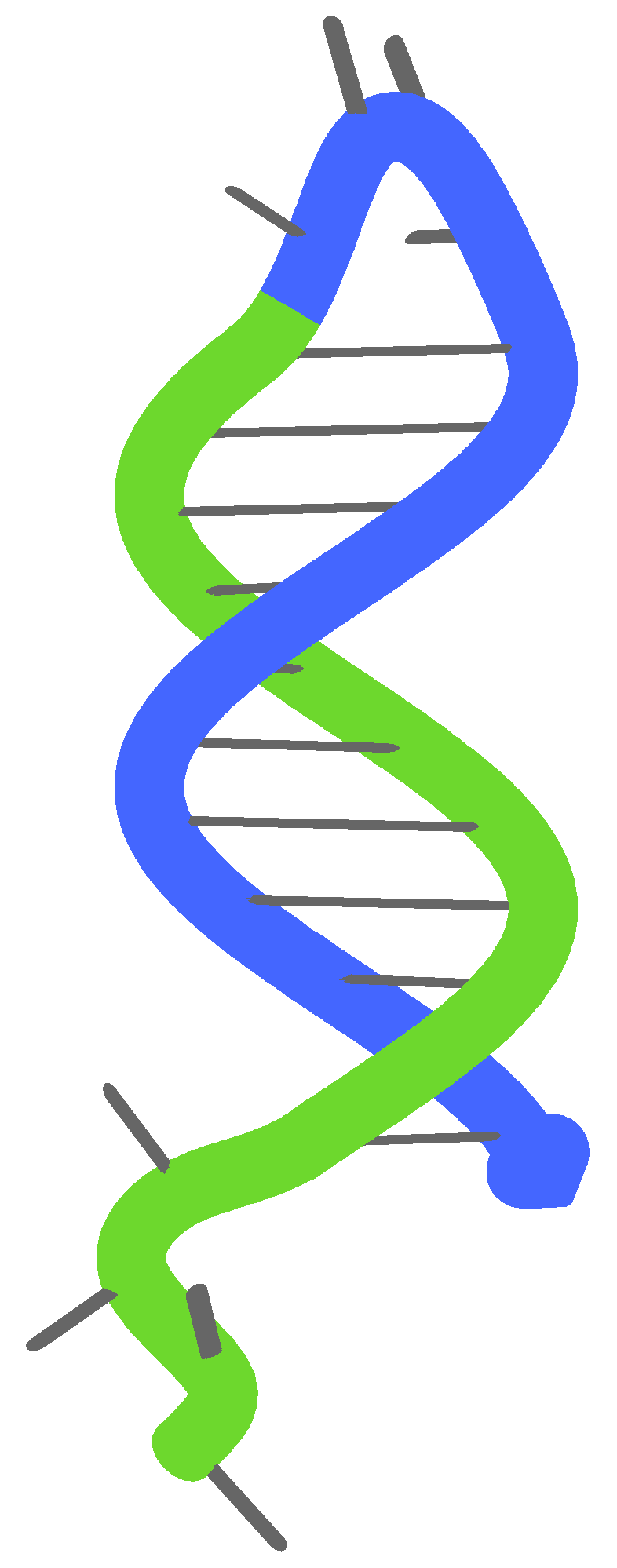
And here is the result...

Wow, that's huge! If you want to be able to size it, you can insert HTML to do so. Here, we would do

<img src="nupack-hairpin.png" alt="NUPACK hairpin logo" style="width: 100px;"/>

And here is the result.

Note that the images are not embedded in the notebooks or in any HTML you output (see below). The images are only linked to in the Jupyter notebook. When submitting your notebook, you also need to submit your images.

Saving your Jupyter notebook as HTML

To save your Jupyter notebook as HTML, just click

File ⟶ Export Notebook As ⟶ HTML

in the menu bar. You should submit your homework via email both as the original Jupyter notebook (.ipynb) and as HTML (.html).